Disney Parks Twitter NLP
NLP Disney Parks brief introduction
Video Presentation at SF Python
Cleaning and Wrangling
- Libraries
- Tweepy
- re
- emoji
- numpy
- bs4
- pandas
- document
- string
-
Twitter sentiment analysis was done for both the Disney Parks. To collect data I used the Twitter API and collected livestream tweets. Collection was done for the Halloween seasonal 2019 and Chinese New Year 2020 events at both Tokyo Disney Resort and Anaheim Disney Resort.
- CNY data collection period Jan 28th - Feb 2nd 2020
- Halloween data collection period Sept 24th - Nov 1st 2019
-
To clean and structure the data the tweepy library was used. Regular expression was used to clean the data and retrieve hashtags,links, mentions and emojis
- Nested dictionaries were pulled out to consolidate the text.
- Date time was formatted
- Numerical data that was used replaced NaNs with 0’s
- Hashtags, Emoticons, Mentions, Links were all put in their own column
-
To do a comparable analysis of Japanese text and English text, word and google translation service was used. After a text sentiment analyzer was applied to the text data.
-
The following libraries/modules were used for sentiment labeling.
- NLTK Vader
- Text Blob
- Asari - was overly positive. Was developed by a python developer on qiita.
- R Sentiment from the cran package.
-
Comparison was made between NLTK, Text Blob and R Sentiment. If two analyzers voted positive then positive was chosen for the text sentiment label. For any remaining ones that a decision couldn’t be reached NLTK Vader was used.
- Geocoder was used to add back in longitude and latitude data for user location.
Exploratory Data Analysis
- Libraries
- seaborn
- matplotlib
- bokeh
- plotly
- Spacy ScatterText
- Folium
- Basemap
- wordcloud
- Counter
-
WordCloud was generated to visualize the top 1000 words.
-
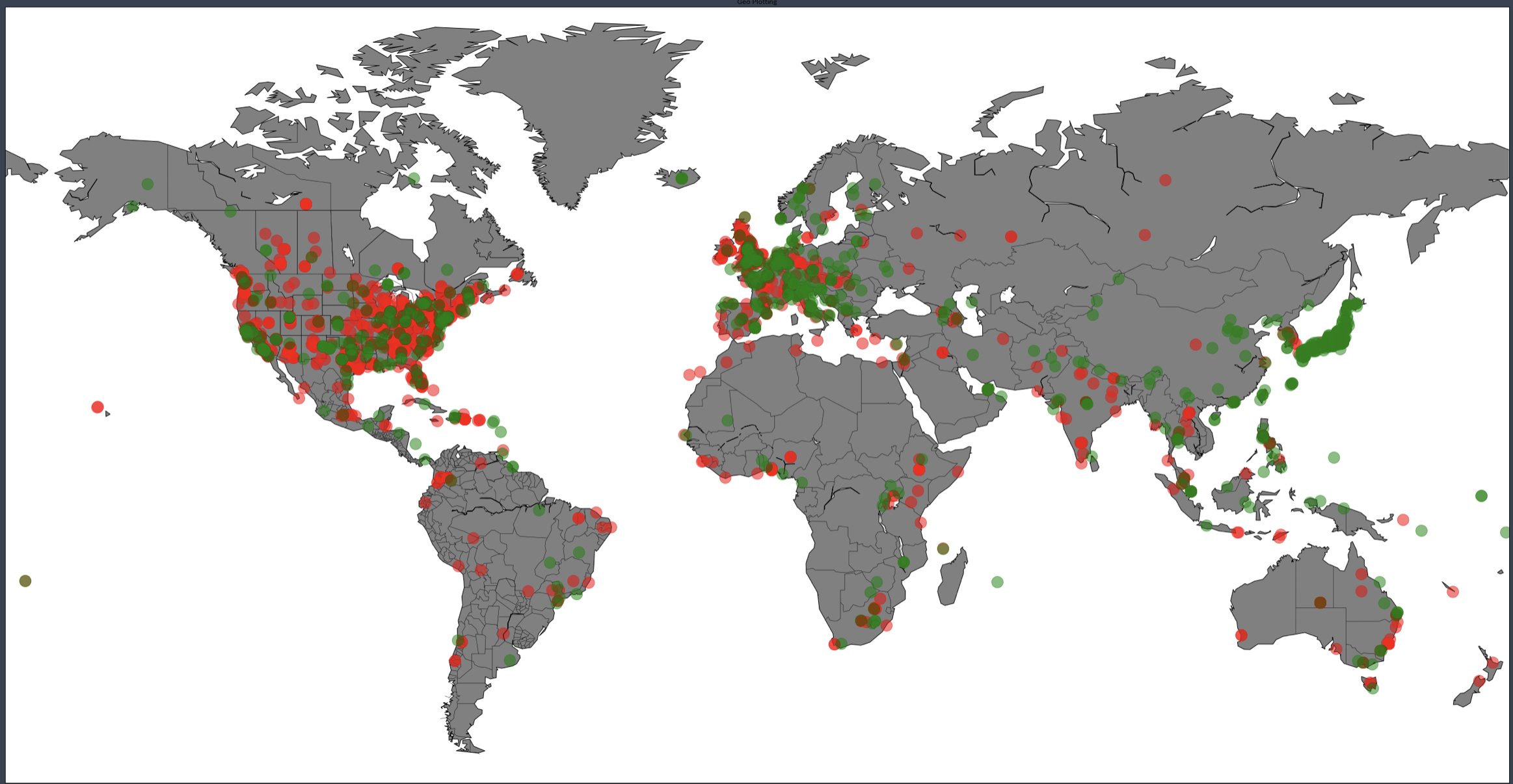
Basemap and Folium interactive map was created to visualize top Disney influencer location.
- Geocoder was used to retrieve longitude and latitude.
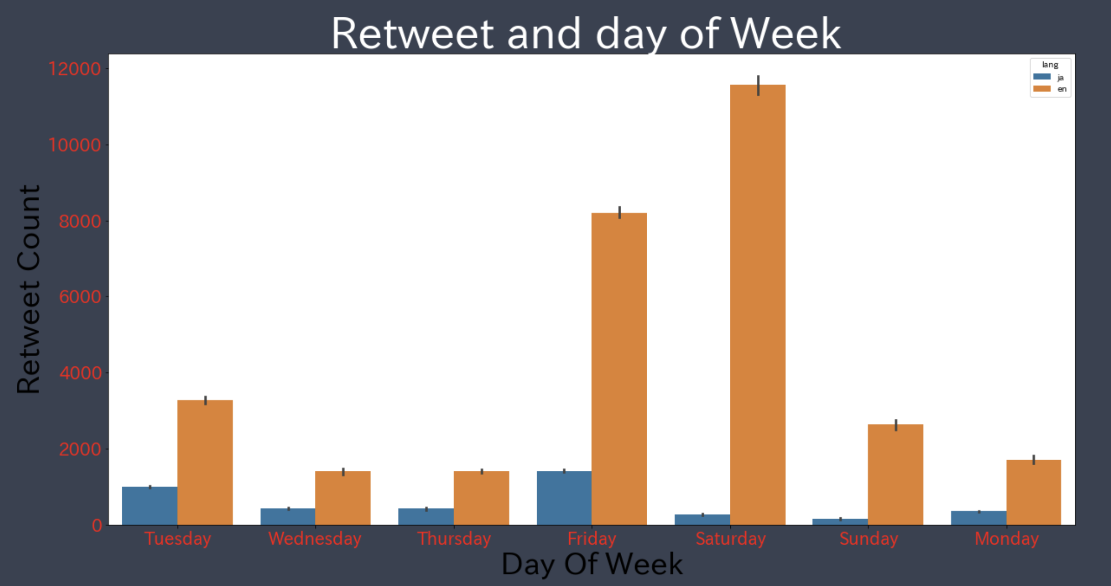
- Seaborn was used to visualize if people tweeted more on the weekend and weekday.
-
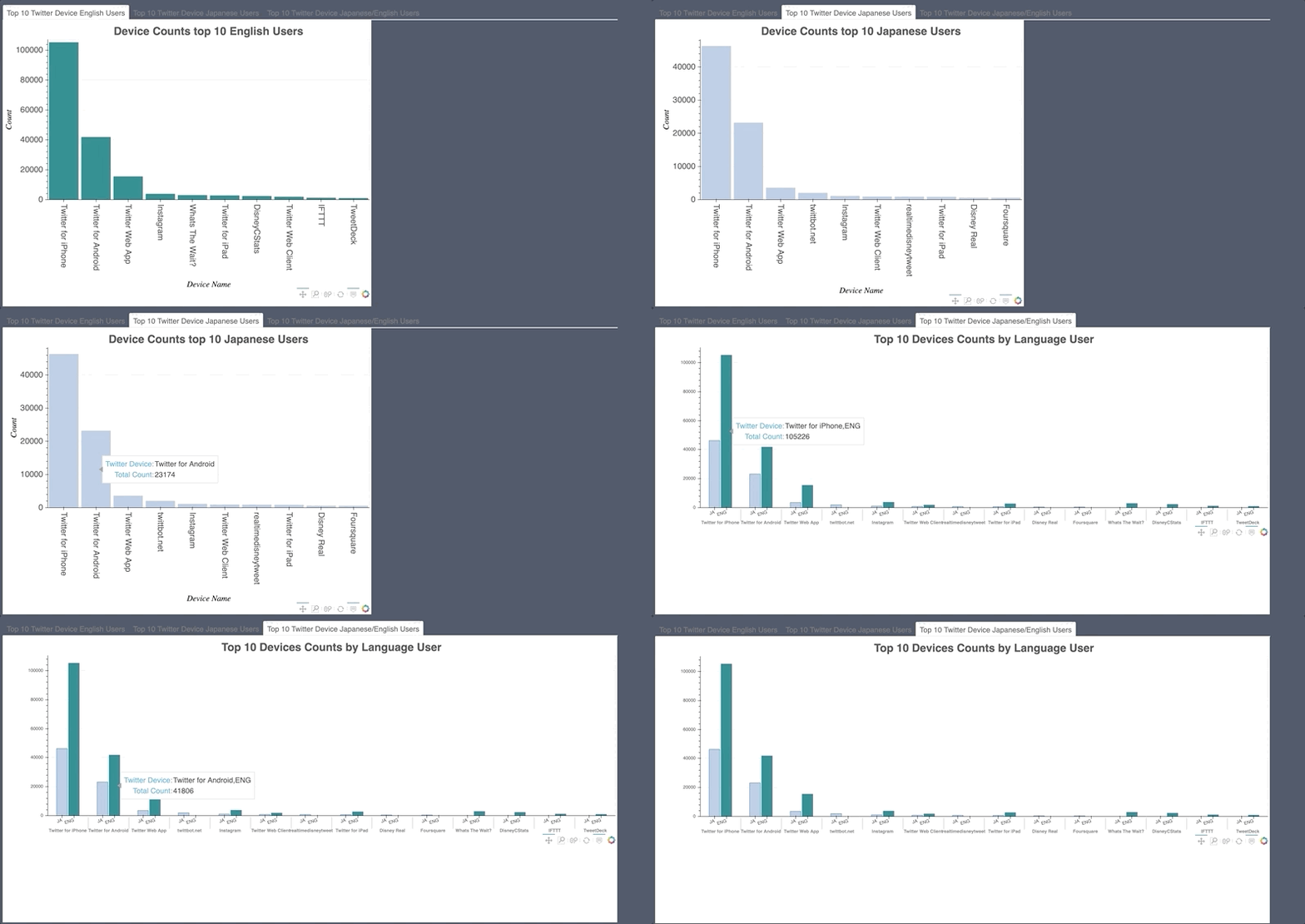
Bokeh was used to visualize hashtag, emoji and mention count. Also, what device people used.
- Noticeable tweet bots found.
- Was also used to count words in countvectorizer document term matrix.
-
Plotly was used to visualize tweet peaks on certain days of the collection period.
-
ScatterText used to visualize word frequency accross Japanese and English documents.
ScatterText Interactive Word Search
#Statistics
- Libraries
- scipy.stats
- nltk
- textblob
- asari
- Mean, median and mode were after finding the compound score text using NLTK Vader.
Vader Compound Score
def vader_compound(sentence):
    score = analyser.polarity_scores(sentence)
    return score['compound']
Text Blob Polarity
pol = lambda x: TextBlob(x).sentiment.polarity
tweets['polarity_tb'] = tweets['clean_text_hashtag_emoji'].apply(pol)
- Used regular expression to classify from the text which parks were being talked about.
- Certain twitter users were mainly one parks influencers included them in search.
Tokyo Disney Search
tweets['disneyTokyo'] = tweets['original_clean_text_hashtag_emoji_mentions'].apply(lambda tweet: word_in_text(r'(disneysea|\
disneytokyo|disneytokyoresort|tokyodisney|tokyodisneyresort|tokyodisneyland|tokyo disneyland|\
tdr_info|東京ディズニーランド|ディズニーランド|東京ディズニーシー|ズニーシー|tdr_now|tdr_md|ディズニーランド|\
tokyo|japan|スプーキーbooパレード|ディズニーランド|TDR|tora0422|スペースマウンテン|ドナルド|マイロ|ミニ|disney_04150420|\
spookybooparade|仮装|カストーディアルアート|パーク|白雪姫|ディズニー|キッズ|コイン|tokyo trip|シー|tds_010904|hinaarare_duffy\
ダッフィー|disney_hokuto|linepay_jp|mikko_20100518|dtr|taa235|tyako_tako_tako|rinarina61423|jr_mmk0620|\
tokyo disney|maihama_line|andrew_minnie_|新幹線|ちゃん|ガチャ|スカイウォーカ|ハロウィン|dontike36|でたよ|舞浜|t_bisco|\
edama_d|moonstar_y_h|tommmdd|2nd887|bom_schedule|ngntrtr|ワンマンズ|fp|doppo_miku|インディージョーンズ|リゾラ|\
ジャングルクルーズ|鹿児島|トラッシュカン|disney6942|noon123hii|h_meika|katsudonminnie|ファストパス発行|natch000|• tokyo|\
花壇|ミッキ|motorsports0908|mjlove_panda|minnie24pre|_disney_mania_|satosan1118mm|海|saiga_d_mickey|koutaman7|\
snow whites scary adventures)', tweet))
Sentiment and Parks
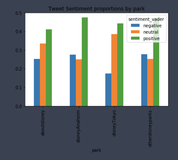
- Mean difference test was done as well as Mann-Whitney U Test non-parametric distribution test.
- Test on Japanese vs English users
- Toyko Disney Resort vs Anaheim Disney Resorts
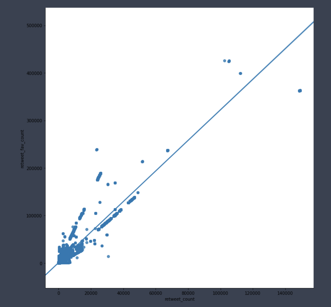
- correlation was visualized
Correlation Retweet and Favorite
Machine Learning
- Libraries
- sklearn
- gensim
- spacy
- nltk
- imblearn
-
Base model evaluation was done to see which best document term matrix to use.
- There was much more English Positive data used RandomOverSampler to balance the data.
Balance data
#Balance the Data
ros = RandomOverSampler(random_state=77)
X_resampled_ros_tf, y_resampled_ros_tf = ros.fit_resample(X_train_vect_tf.values, y_train.values)
print(sorted(Counter(y_resampled_ros_tf).items()))
- Feature engineering and selection
- tweet length
- R emotion range
- capitalize count
- punctuation count
- emoji count
- hashtag count
- Thought of using box cox transformation to normalize the features however believed central limit theorem should hold.
Box Cox Transformation
#Box-cox transformation for emoji count
for i in [1,2,3,4,5]:
    plt.hist(df3['emoji_count']**(1/i),bins =8)
    plt.title('Transformation : 1/{}'.format(str(i)))
    plt.show()
- word2vec showed similarity in words

- model was then tuned using RandomizedSearchCV 1000 max features used to speed up fit time.
- xgboost
- knn
- naive bayes
- logisitic regression
- random forest
- data was split using train test split to test which one performed the best
- random forest and naive bayes were selected
-
min_df and max_df and max features was then tested to see which combination using the two models would give the best metrics.
-
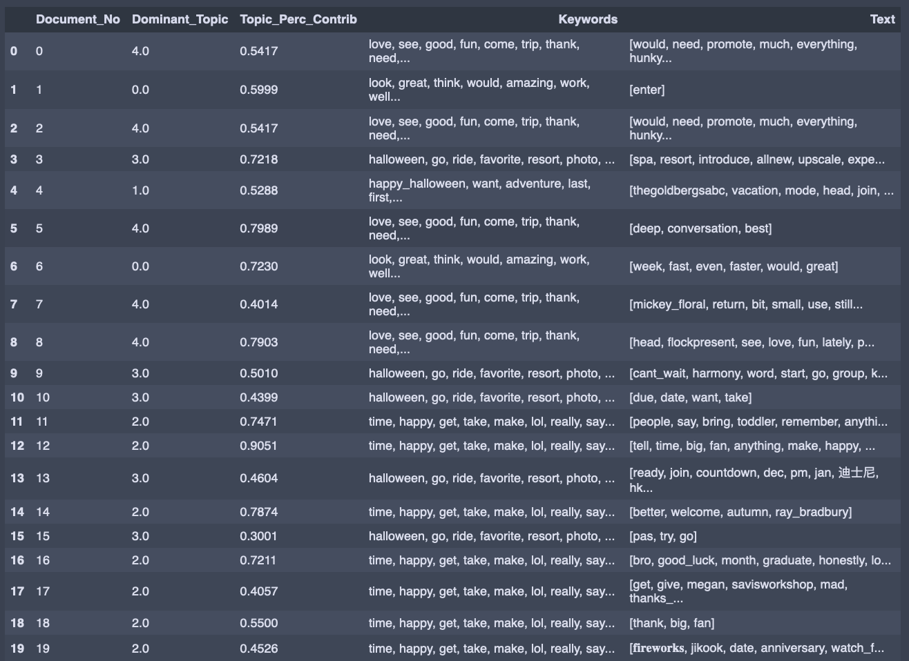
LDA was done on tweets separated by sentiment to see if topics could be found.
- Japanese negative
- Japanese positive
- English negative
- English positive
Dominant word per document English Positive
- Full write up, blog post and github link can be found below.
