Disney NLP: Analysis of Tokyo and Anaheim Disney Resorts

Intro

• The project was inspired by my summer trip to Tokyo Disneyland. Researching guides on youtube there was a huge number of Youtubers, people on reddit, twitter and other forms of media claiming Tokyo Disney Resort specifically Tokyo Disney Sea was the best Disney park. The park that would make Walt Disney proud.

• The business use of doing NLP for both Disney resorts would be to help Imagineers come up with new decorative themes for the park during seasonal events. By seeing trends of what people liked and disliked it can help relay information to Disney’s business partners of what worked and didn’t work.

• So what is an Imagineer you might ask?

• Imagineers are in charge of dreaming, designing and building Disney theme parks, attractions, cruise ships, resorts etc. Basically, they’re about live entertainment. They create things you can see and touch and smell, experiences that you can walk right into. They’re the ones who create the experience and allow visitors to emerge themselves into the world of Disney. For example, the new Galaxy Edge now allows Star Wars fans for a place to gather and enjoy themselves on Batuu.

Twitter API Data Collection

• Data was collected through the Twitter API from September 24th, 2019 to November 1st, 2019.

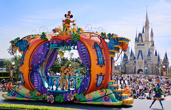
• Tokyo Disney - Spooky Boo Halloween Parade

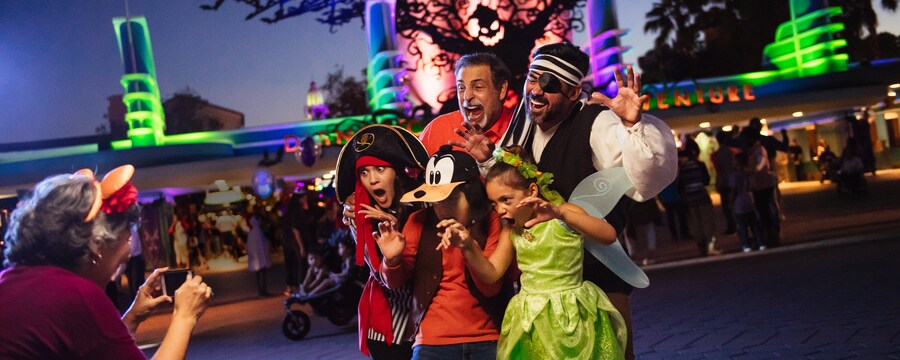
• Anaheim Disney - Oogie Boogie Bash

• The following was searched for using Tweepy and the Twitter API

Disney Anaheim	Disney Tokyo
disneylandresort	disneysea
disneyland	disneytokyo
disneyresort	disneytokyoresort
californiaadventure	tokyodisneyresort
downtowndisney	tokyodisneyland
disneyanaheim	東京ディズニーランド
dca	ディズニーランド
disneylandanaheim	東京ディズニーシー
disneycalifornia	ズニーシー
californiadisney	tdr_now
	tdr_md

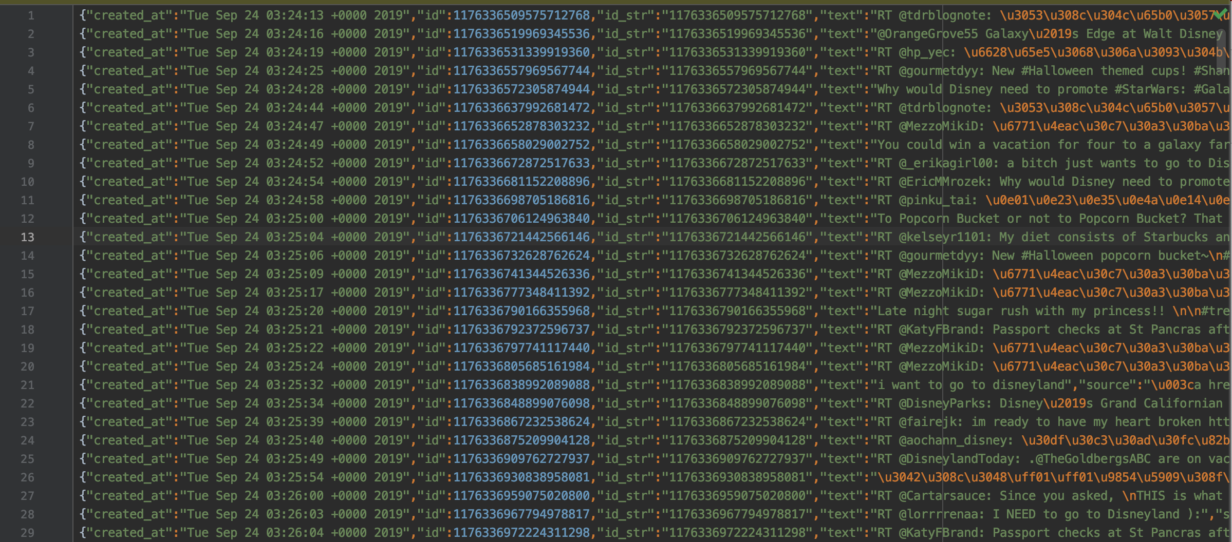
• Tweepy after collecting from Sept 24th, 2019 to Nov 1st, 2019 throughout the day returned a json file.

Tweepy Json File

Data Wrangling/Cleaning

Tweepy separate collected tweets into four separate nested dictionaries.

• extended_tweet
• extended_entities
• retweeted_status
• text
• quoted_status

Data Wrangling Highlights

Getting Nested Dictionaries

df['ex_tw_full_text'] = [d.get('full_text') if type(d) == dict else np.nan
                          for d in df['extended_tweet']]

Combining text field into one

#combining text columns tweets
df['text'] = df['text'].replace(np.nan,'')
df['len_text'] = df['text'].apply(len)
df['combo_text'] = np.where(df['len_text'] < 140, df['text'], df['ex_tw_full_text'])
df['combo_text'] = df['combo_text'].replace(np.nan,'')

#combining text columns retweets
df['rt_text'] = df['rt_text'].replace(np.nan,'')
df['rt_len'] = df['rt_text'].apply(len)
df['rtcombo_text'] = np.where(df['rt_len'] < 140, df['rt_text'], df['rt_full_text'])
df['rtcombo_text'] = df['rtcombo_text'].replace(np.nan,'')

#combining retweets and tweets
df['rtcombo_len'] = df['rtcombo_text'].apply(len)
df['full_text'] = np.where(df['rtcombo_len'] == 0, df['combo_text'], df['rtcombo_text'])

Geocoder API for missing location data

from opencage.geocoder import OpenCageGeocode
from pprint import pprint
key = # get api key from:  https://opencagedata.com
geocoder = OpenCageGeocode(key)


en_lat = []   # create empty lists
en_long = []

for x in en_loc3000.user_location: # iterate over rows in dataframe
    try:
        query = x
        results = geocoder.geocode(query)   
        lat = results[0]['geometry']['lat']
        long = results[0]['geometry']['lng']
        en_lat.append(lat)
        en_long.append(long)
    except IndexError:
        en_lat.append(np.nan)
        en_long.append(np.nan)

Word Document Back to Python after Word/Google Translation Japanese Text

import io
import csv
from docx import Document

def read_docx_tables(filename, tab_id=None, **kwargs):
    def read_docx_tab(tab, **kwargs):
        vf = io.StringIO()
        writer = csv.writer(vf)
        for row in tab.rows:
            writer.writerow(cell.text for cell in row.cells)
        vf.seek(0)
        return pd.read_csv(vf, **kwargs)

    doc = Document(filename)
    if tab_id is None:
        return [read_docx_tab(tab, **kwargs) for tab in doc.tables]
    else:
        try:
            return read_docx_tab(doc.tables[tab_id], **kwargs)
        except IndexError:
            print('Error: specified [tab_id]: {}  does not exist.'.format(tab_id))
            raise

Sentiment labeler 3 sentiment analyzer voting tiebreaker

#Creating the tie breaker between textblob,vader and r_sentiment
test = np.where((df3['vader_score_word'] == df3['tb_word']), df3['vader_score_word'], 'not sure')
test2 = np.where((df3['tb_word'] == df3['r_sentiment']), df3['tb_word'], 'not sure')
test3 = np.where((df3['vader_score_word'] == df3['r_sentiment']), df3['vader_score_word'], 'not sure')


test = pd.DataFrame(test)
test.rename(columns = {0:'vaderVstb'}, inplace = True)
test['tbVsr'] = test2
test['vaderVsr'] = test3


t2 = np.where(test['vaderVstb'] == 'not sure', test['tbVsr'], test['vaderVstb'])
t2 = pd.DataFrame(t2)
t2.rename(columns = {0:'compare1'}, inplace = True)
t2['compare2'] = np.where(t2['compare1'] == 'not sure', test['vaderVsr'], t2['compare1'])

#Remaining 5510 rows still not sure.  Since vader analyzes emoticons better we will use vader as the final tie breaker
t2['compare3'] = np.where(t2['compare2'] == 'not sure', df3['vader_score_word'], t2['compare2'])
df3.loc[:,'label'] = t2.loc[:,'compare3']

• The Data Frame used for EDA and statistical analysis had 270850 rows and 56 columns.
• Machine learning data preparation had 87510 rows and 17 columns.
• Japanese text was translated using Office 365.
• R Sentiment, NLTK Vader and TextBlob was used to label text sentiment.

Exploratory Data Analysis

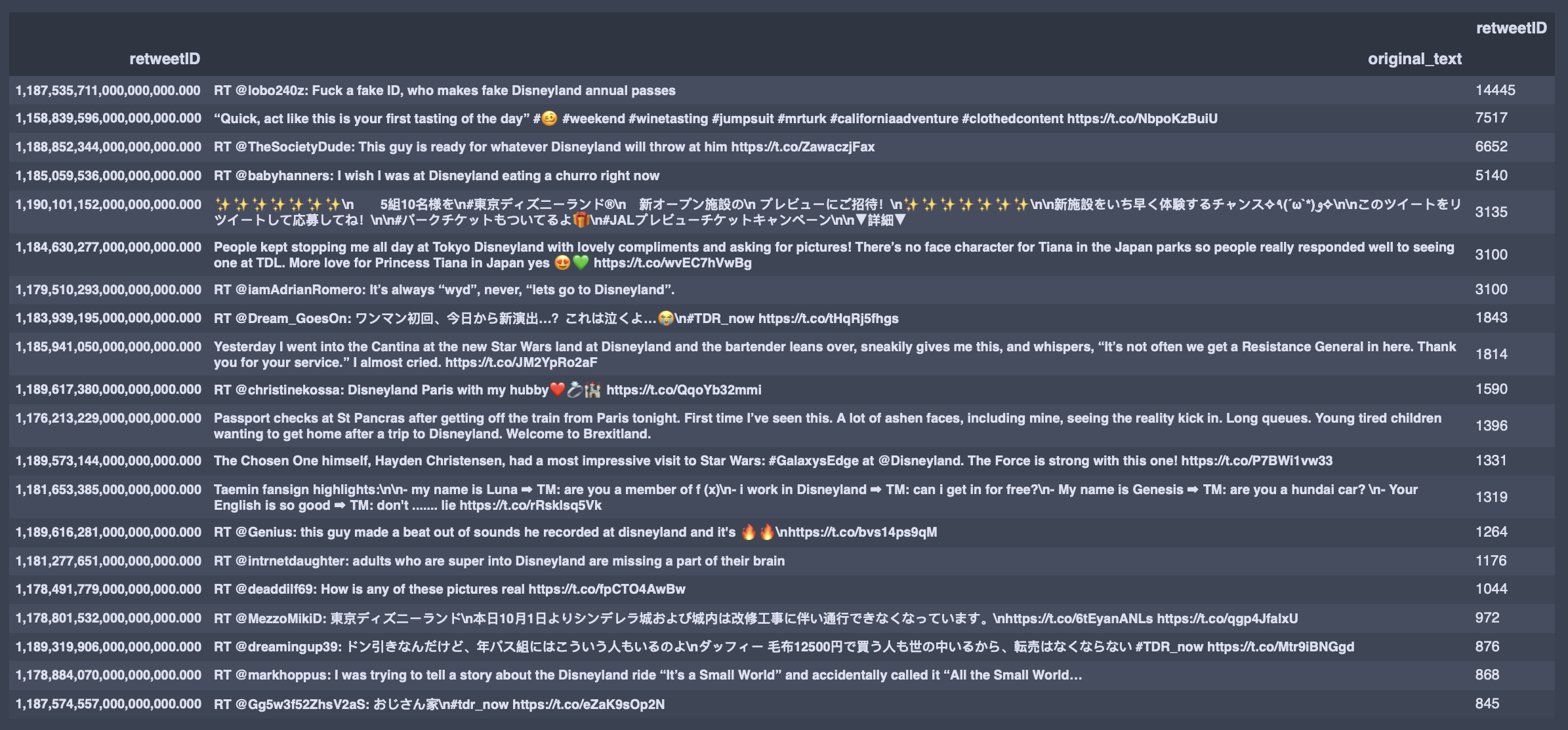
Most Retweeted During the collection period

English Twitter User WordCloud

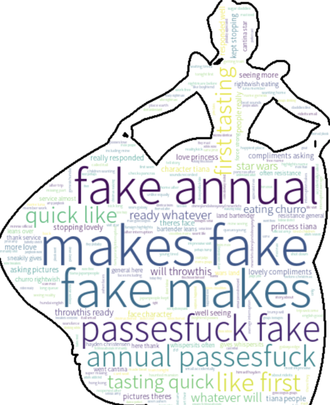
• The most common words are fuck and annual pass.

Japanese Twitter User WordCloud

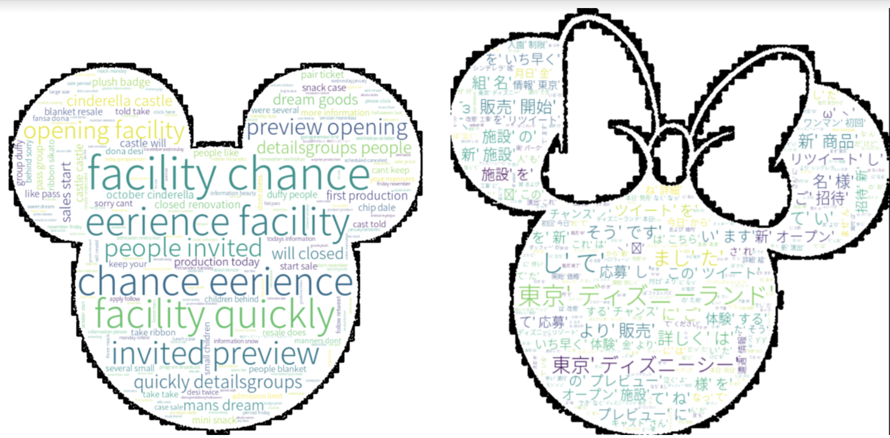
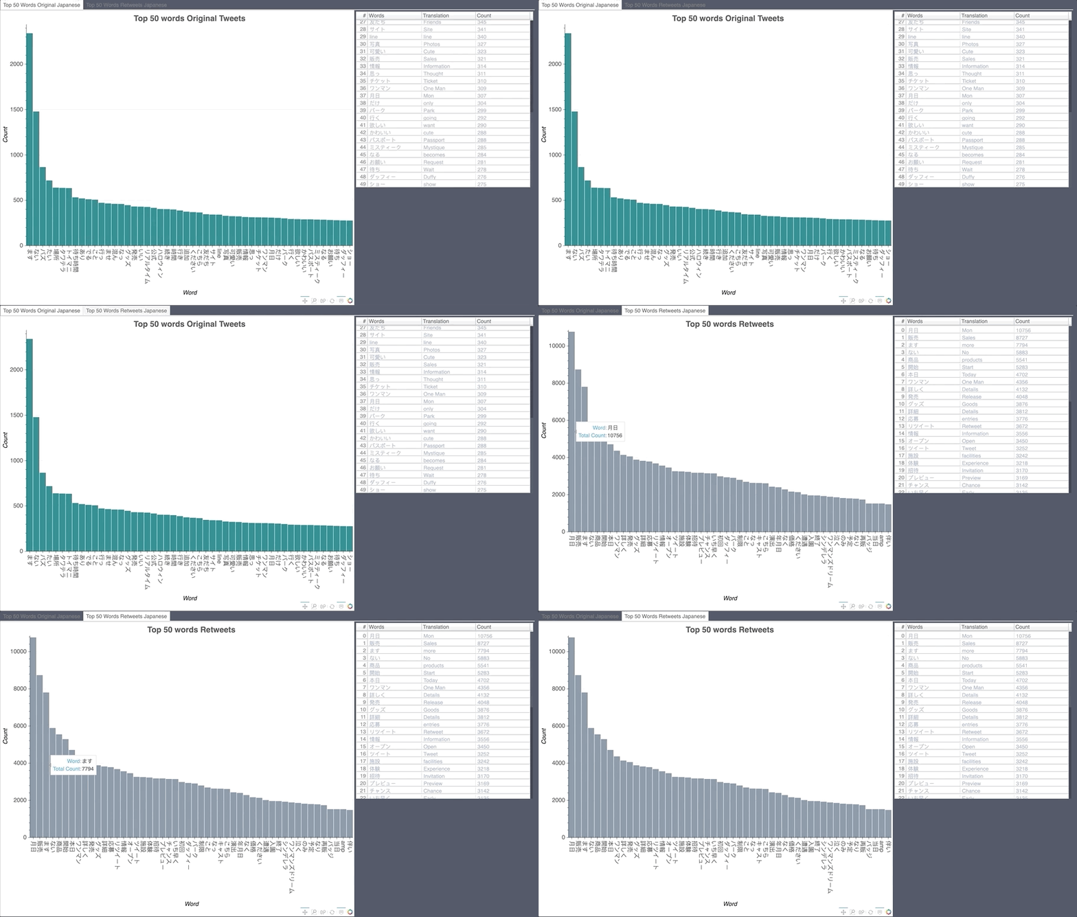
• Things like the experience, lottery tickets for the show One Mans Dream was being talked about the most in the Japanese text WordCloud visualization.

Tweet Peaks For English Users

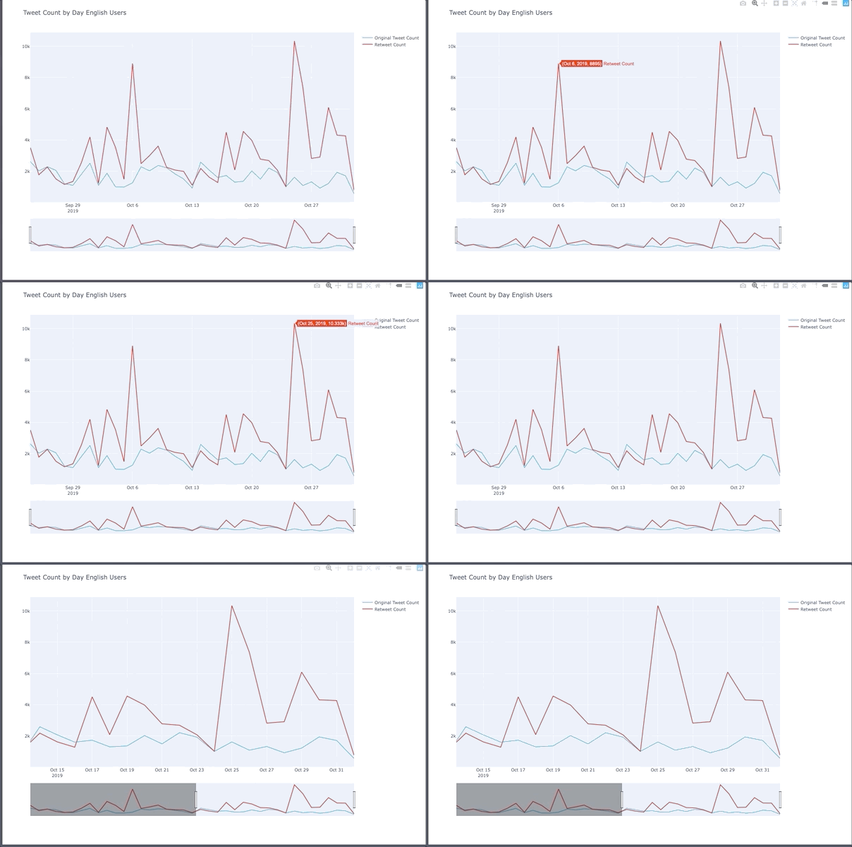
• Oct 6th was Gay Days Anaheim.
• 25th was the weekend before halloween and people celebrated before the 31st which was a Thursday in 2019.

Tweet Peaks For Japanese Users

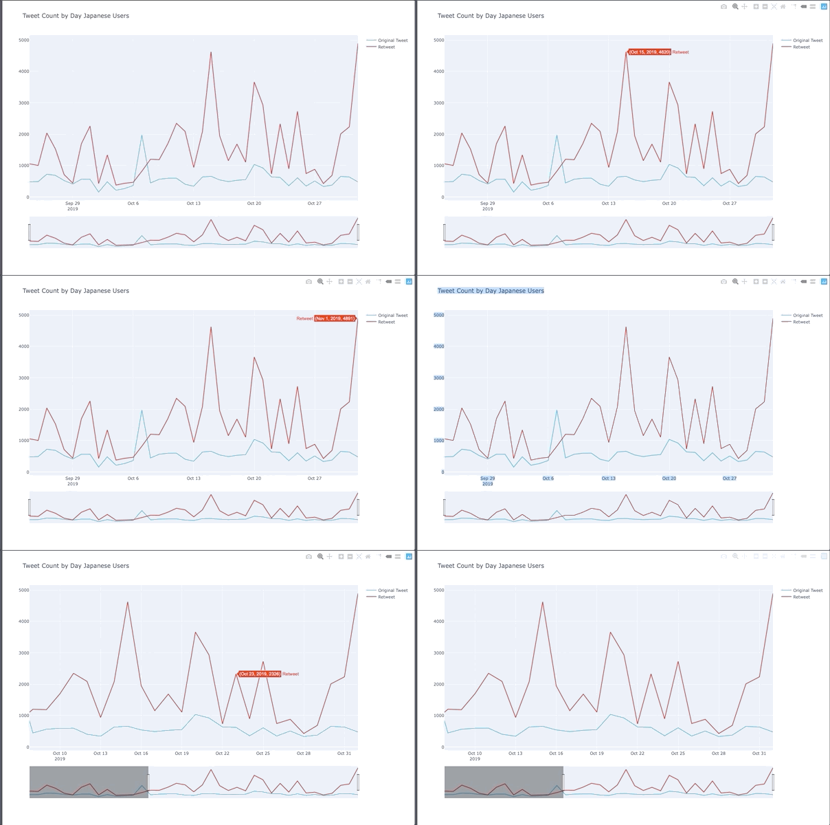
• Tweet count spiked up on the 15th for the Japan Airline promotion
• 20th people were tweeting about One Man’s Dream 2 ending
• November 1st was the day after Halloween

English Hashtag/Emoji/Mention Count

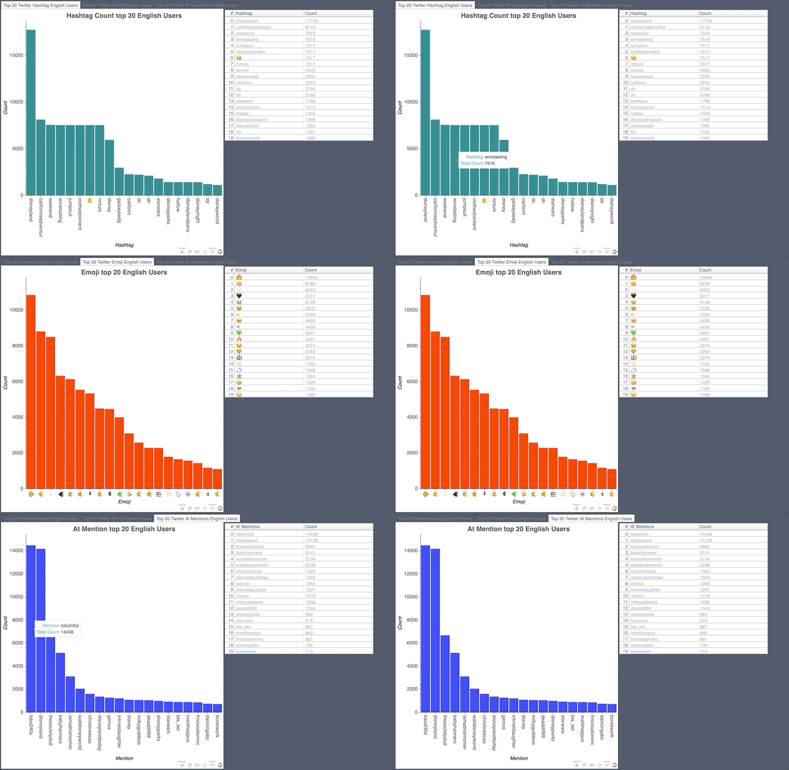
• The pumpkin of course was the highest used emoji during the Halloween event.
• The disgusting face showed up in the hashtags as there was a measles scare at Disney Land.

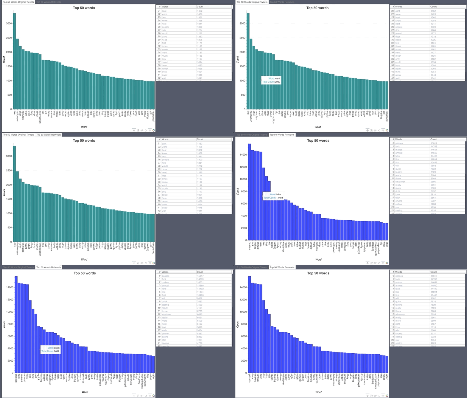
English Word Count

Japanese Hashtag/Emoji/Mention Count

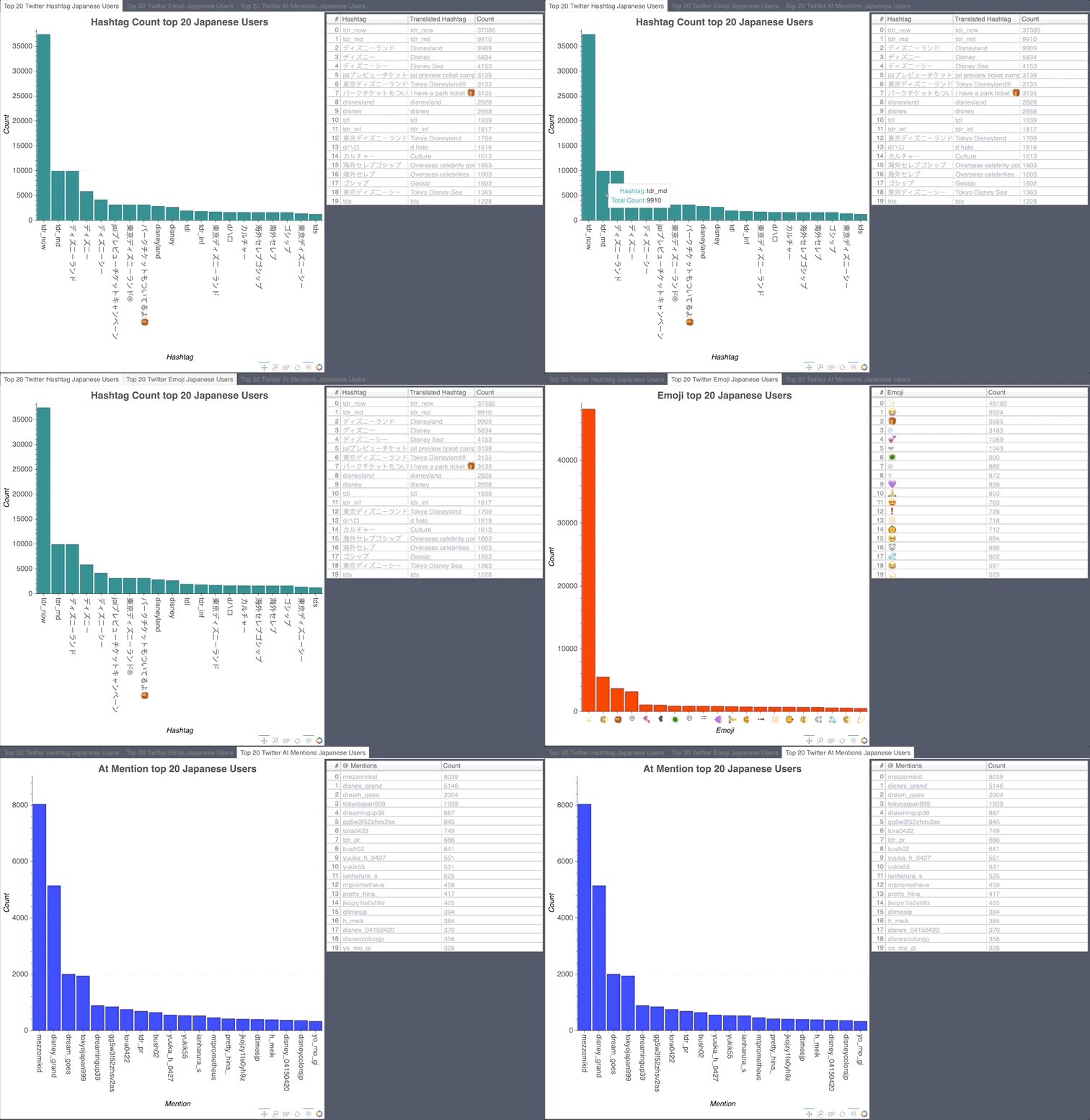
• Japan airlines ran a promotion giving away free Disney Land tickets, there were a lot of stars in their tweet.
• tdr_now talks about what is happening right now at Tokyo Disney Resort. tdr_md is Tokyo Disney Resort Merchandise.

Japanese Word Count

Influencer Map English

• Most English twitter Users were in Europe and America.

Influencer Map Japanese

• Most Japanese Twitter users were in Japan or in America.

Twitter Interactive Influencer Map

• ScatterText part of Spacy, allows you to look up certain words and shows you in which document in the corpus the word shows up in.
• Japanese documents were compared with English.

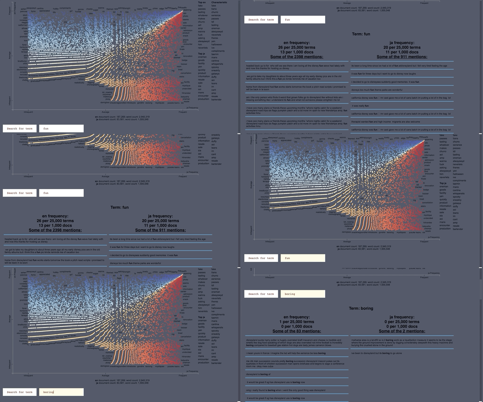
ScatterText Interactive Word Search

Statistics

Difference Between Means

Do Japanese twitter users have more or equal positive sentiment towards the Disney parks than English twitter users?

H₀ : English and Japanese Twitter users have the same Text Blob polarity or Vader Compound with their sentiment to the Disney Parks during the Halloween event.

H₀ : μ₁ ≠ μ₂

H_A : English and Japanese twitter users have different Text Blob polarity or Vader Compound with their sentiment towards the Disney Parks during the Halloween event.

H_A : μ₁ ≠ μ₂

alpha : 0.05

Params:	Vader Compound Score	Text Blob Polarity
Mean difference	-0.1117	-0.0101
t-stat	47.4353	7.9732
p-value	0.000	0.000

Params:	Vader Score Mean	Text Blob Score Mean
English	0.114	0.543
Japanese	0.226	0.482

NLTK Vader Distribution

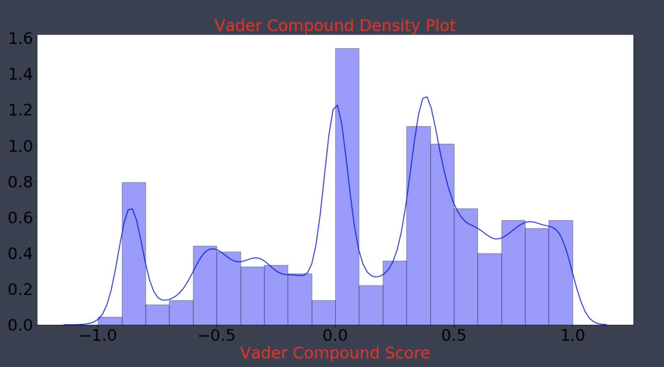
• Distribution wasn’t normal after using the Shapiro Wilk test, however central limit theorem should hold.
• Non-Parametric test Mann-Whitney U was used to validate.

Mann-Whitney U Test non-parametric distribution test

• Tests whether the distributions of two independent samples are equal or not.

H₀ : the distributions of both samples are equal.

H_A : the distributions of both samples are not equal.

Japanese Twitter users vs English Twitter Users

Params	Vader Compound Score	Text Blob Polarity
stat	4493129062.500	4867484730.500
p-value	0.000	0.000

Japanese and English twitter users have different sentiment towards Disney on twitter. Both p-values were far below 0.05. TextBlob gave a higher score for English users, however NLTK Vader is more accurate in interpreting social media sentiment.

Correlation Matrix

• Correlation is high between favorite count and retweet count.

Machine Learning

• The goal here is to create a classifier that can classify negative and positive and between Japanese and English. After classification hopefully topic models can be generated to give insight to Imagineers or Disney partners.

Preprocessing Text Steps

1. Remove amp,&, /n, lxml
2. Remove href
3. Remove @ mentions
4. Remove RT
5. Lemmatize
6. Remove punctuation
7. Remove short words less than 2 characters
8. Remove special Japanese Punctuation
9. Tokenize

stopwords = nltk.corpus.stopwords.words('english')
wn = nltk.WordNetLemmatizer()
punc = lambda x: re.sub("!|,|\?|\'|-|\"|&|。|\)|\(|！|，|\.*|/|\[|\]|\u2026|\d|:|~|、|？|☆|’|– |【|】|「|」|《|》|※| “|”|＊|→||[\b\.\b]{3}||@||@ |#|# |", '',x)

#Clean
def clean_text(soup):
    soup = BeautifulSoup(soup, 'lxml')
    souped = soup.get_text()
    stripped = re.sub(r'https?://[A-Za-z0-9./]+', '', souped)
    words = stripped.split()
    mention = [word for word in words if not word.startswith('@')]
    RT = [word for word in mention if not word.startswith('RT')]
    text = " ".join([wn.lemmatize(word) for word in RT if word not in stopwords])
    punct = "".join([word.lower() for word in text if word not in string.punctuation])
    short_words = ' '.join([w for w in punct.split() if len(w)>2])
    ja_punct = ''.join([punc(word) for word in short_words])
    tokens = re.split('\W+', ja_punct)
    return (" ".join(tokens)).strip()

The following features were engineered.

• Tweet Length
• Capitalization Count
• Punctuation Count
• Hashtag Count
• Emoji Count
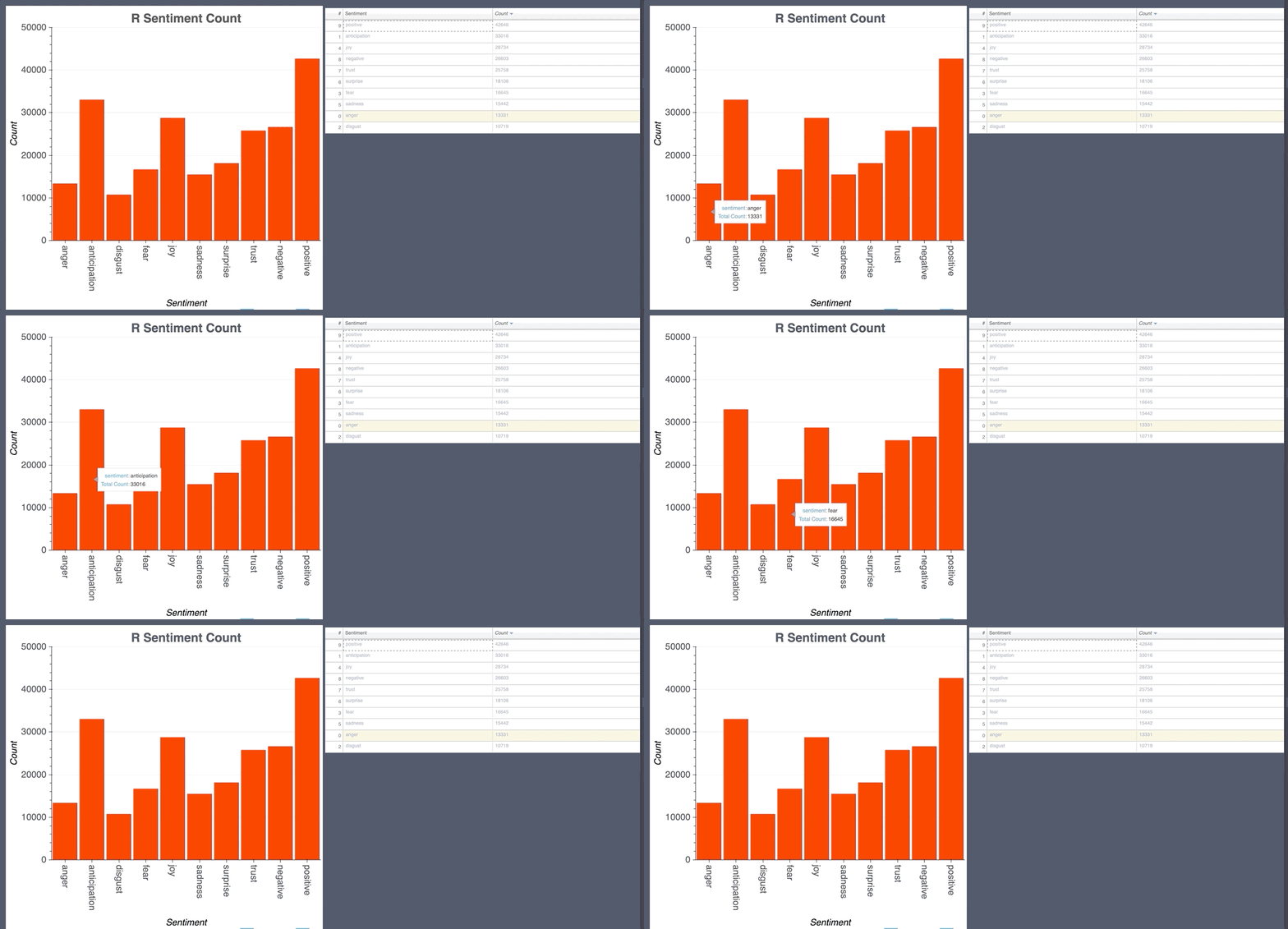
• R Sentiment Emotion

Random Forest Classifier CountVectorizer

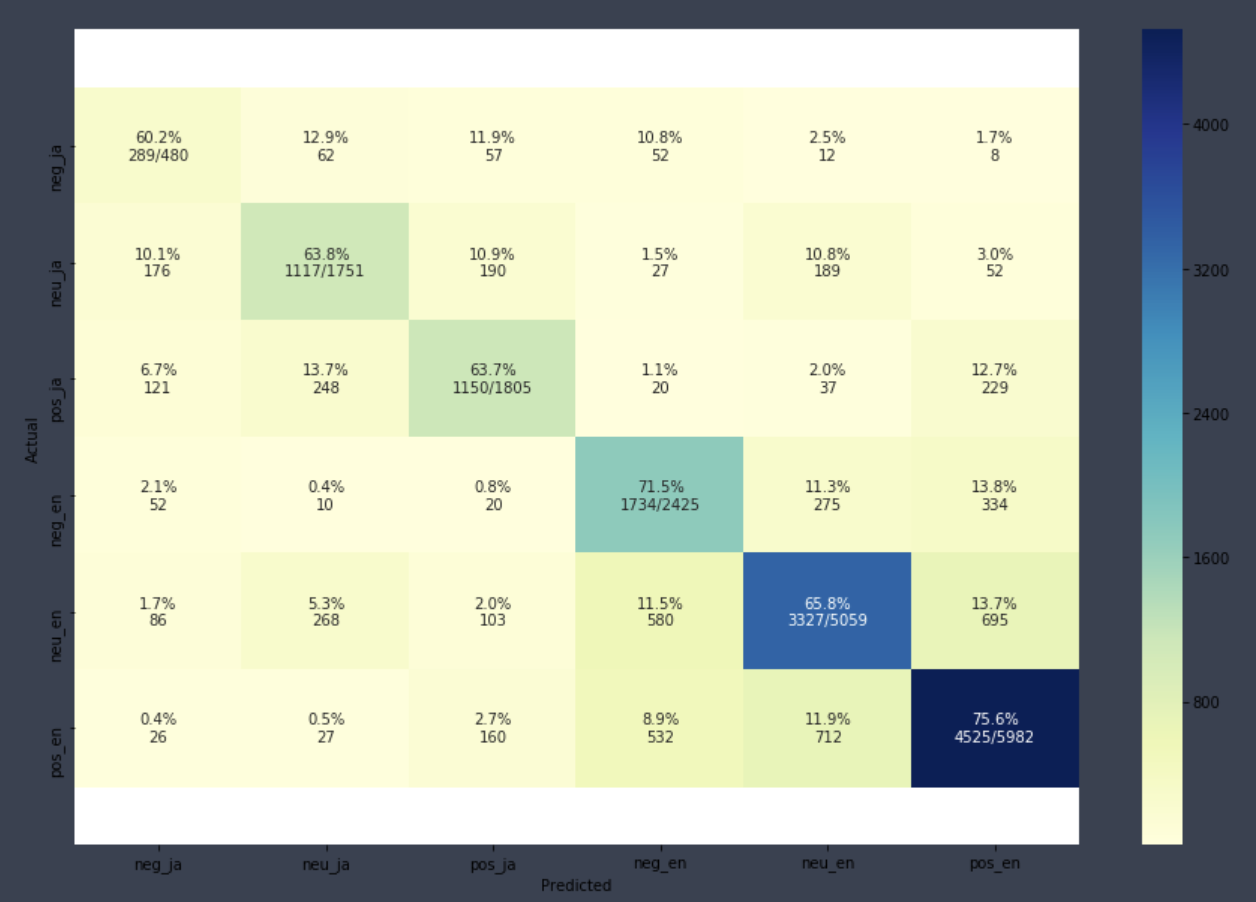
• Labels for prediction are 0-ja negative, 1-ja neutral, 2-ja positive, 3-en negative, 4-en neutral, 5-en positive.

Hyperparameter Tuning

rf_clf = RandomForestClassifier()

hyperparameters = {
    'n_estimators': range(50,1000,100),
    'max_depth': [5,50,100, 200, 300, 400, 500],
    'max_features': ['auto', 'sqrt', 'log2']
}

clf = RandomizedSearchCV(rf_clf, hyperparameters, cv=5, n_jobs=-1,
                         n_iter = 10, random_state = 77)
%time rf_cv_fit = clf.fit(X_count_r, y_r)

Random Forest Feature Importance

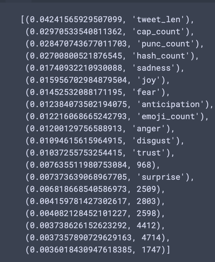
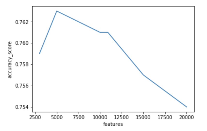
• MaxFeatures of 5000 was chosen with a CountVectorizer document term matrix.

Features vs Accuracy Score

Random Forest Final Model

#Instantiate our model
rf = RandomForestClassifier(n_estimators = 650, max_depth = 500, max_features = 'log2',
                            n_jobs=-1)

#Model Fit
start = time.time()
rf.fit(X_resampled_ros, y_resampled_ros)
end = time.time()
fit_time = (end - start)

#Model Predict
start = time.time()
y_pred = rf.predict(X_test_vect)
end = time.time()
pred_time = (end - start)

Metrics

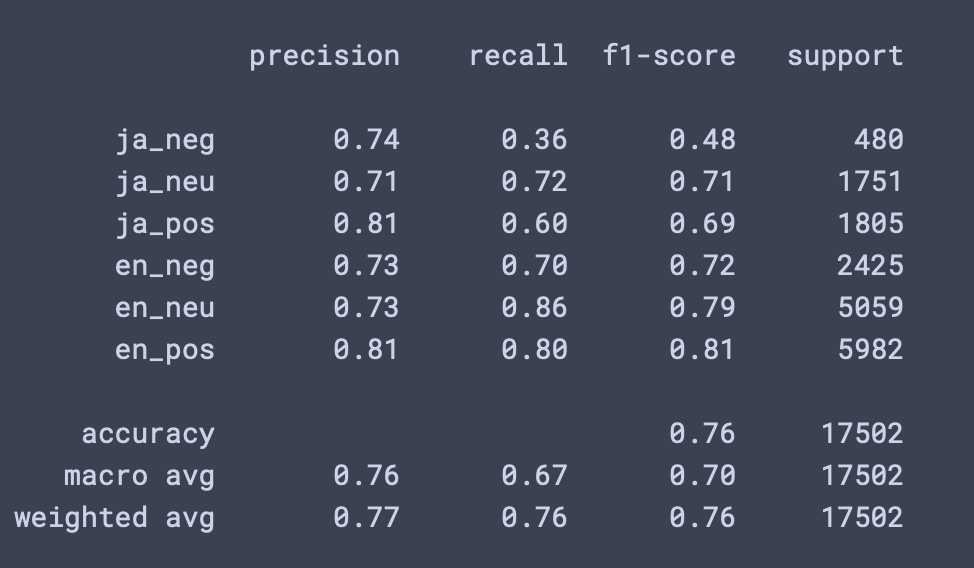
Confusion Matrix

LDA Topic Modeling

• Now that we have a model that can classify sentiment.
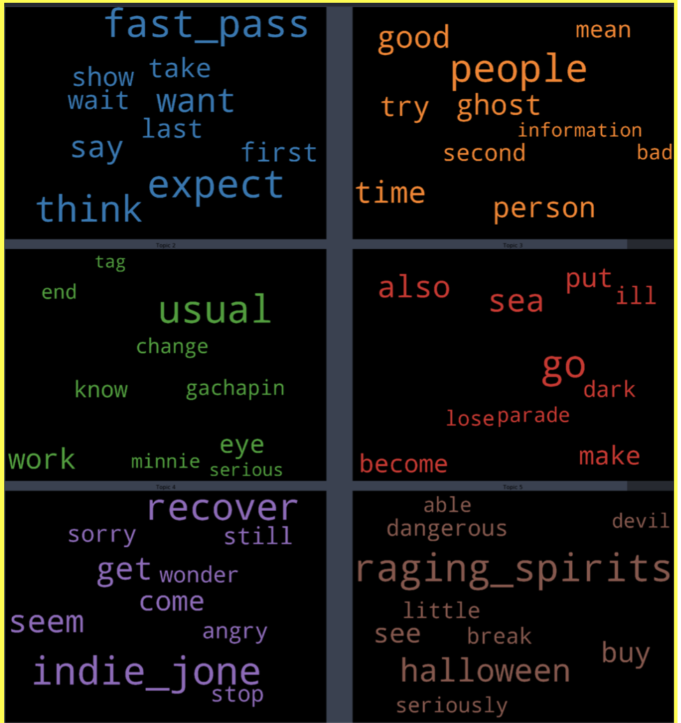
• Want to take positive and negative sentiment and create topics to relay information to the Imagineers or Disney merchandise partners.

Latent Dirichlet Allocation Model

lda_model = gensim.models.ldamodel.LdaModel(corpus=corpus,
                                           id2word=id2word,
                                           num_topics=4,
                                           random_state=777,
                                           update_every=1,
                                           chunksize=10,
                                           passes=10,
                                           alpha='symmetric',
                                           iterations=100,
                                            per_word_topics=True)

WordCloud Topic Negative Japanese

pyLDAvis Negative Japanese

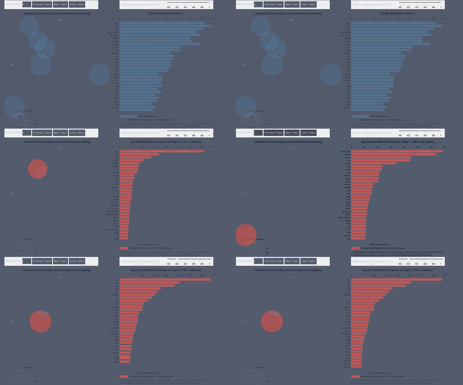
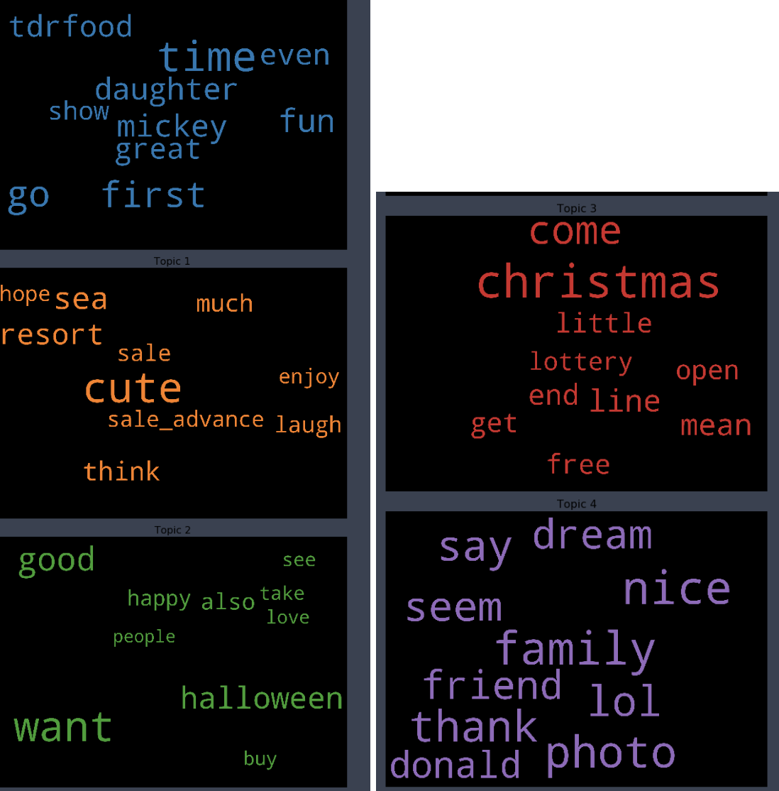
WordCloud Topic Positive Japanese

pyLDAvis Positive Japanese

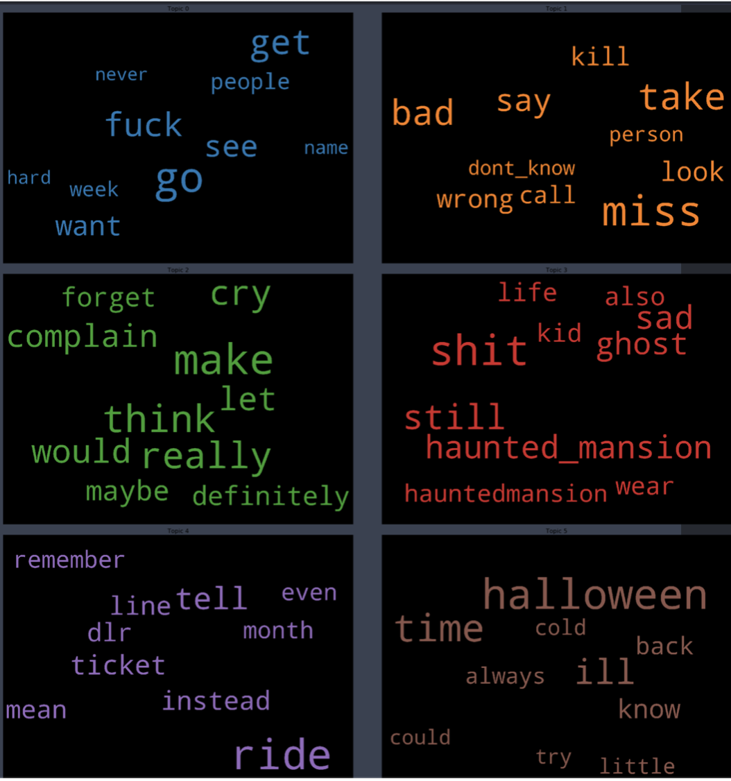
WordCloud Topic Negative English

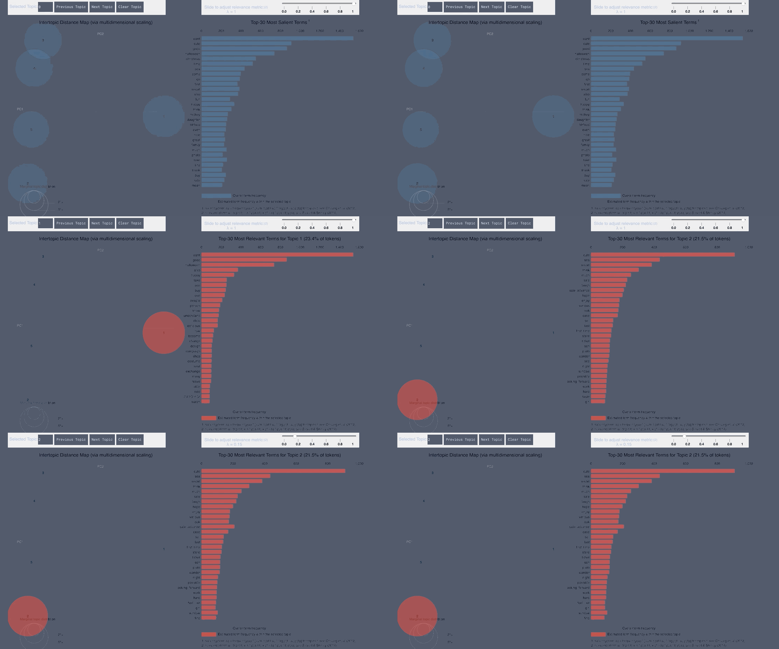
pyLDAvis Negative English

WordCloud Topic Positive English

pyLDAvis Positive English

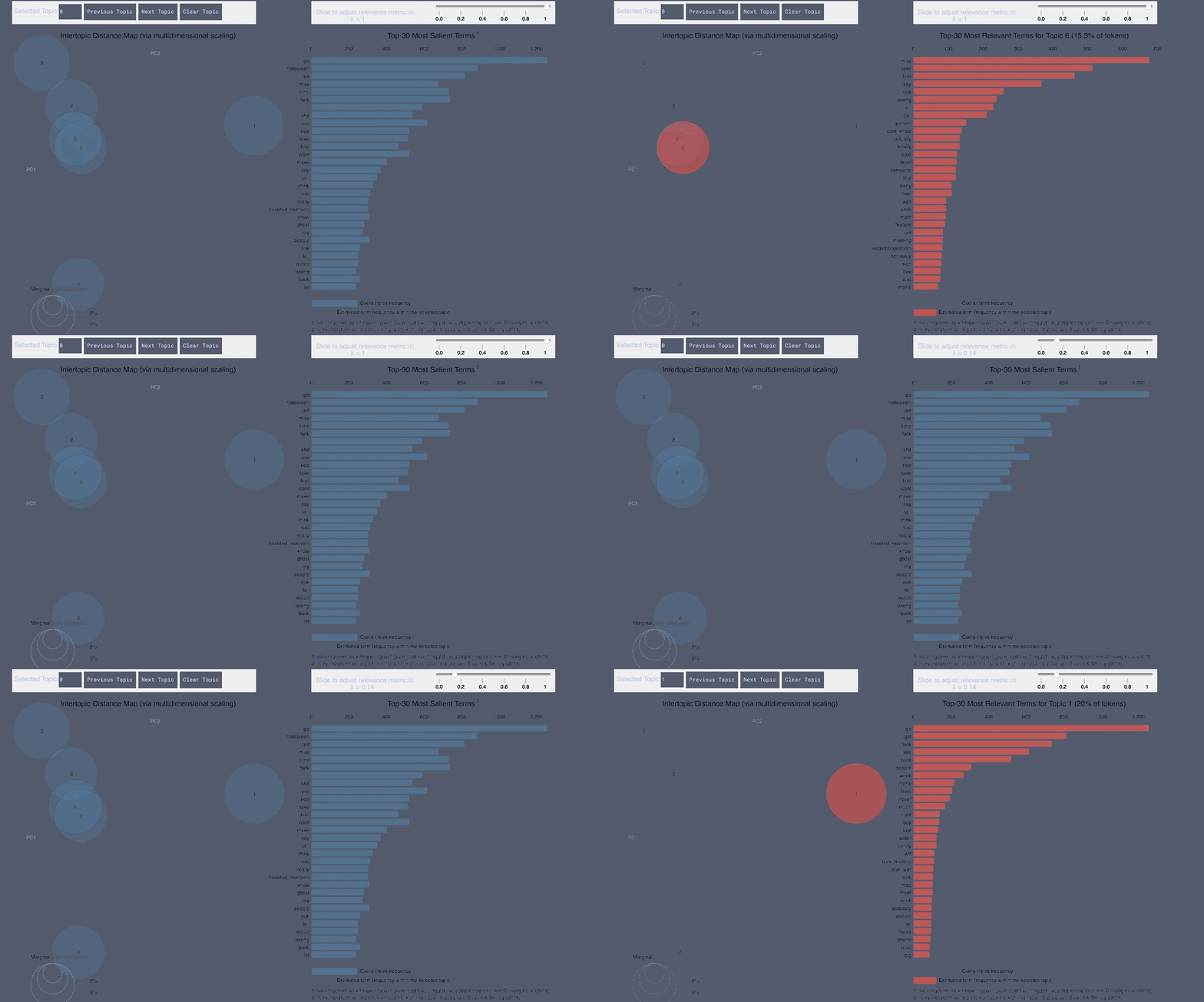
• From the Japanese word cloud we can see topics like family and the last show of One Man’s Dream forming
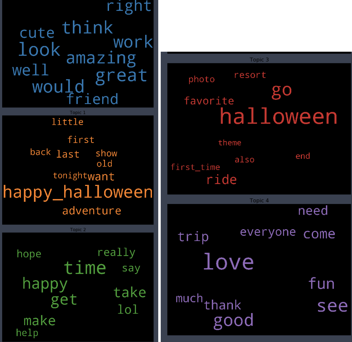
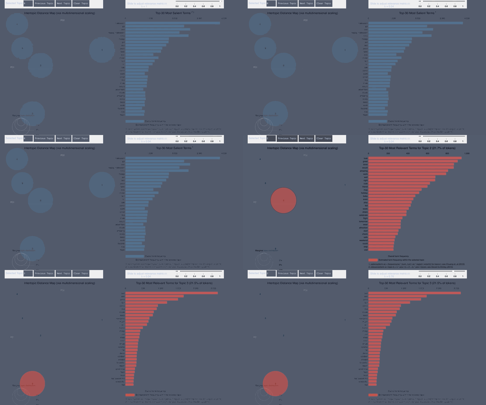
• From the English tweets we can see topics about the cold and long lines and Halloween celebration forming.

Model in Action for Chinese New Year Event Tweets

• Below is a link of the sentiment classifier model
• It will collect twitter data from the Twitter API
• Clean the data
• Do some visualization of word count
• Then run a classifier and topic builder

Disney NLP Model Start to Finish

CNY Confusion Matrix

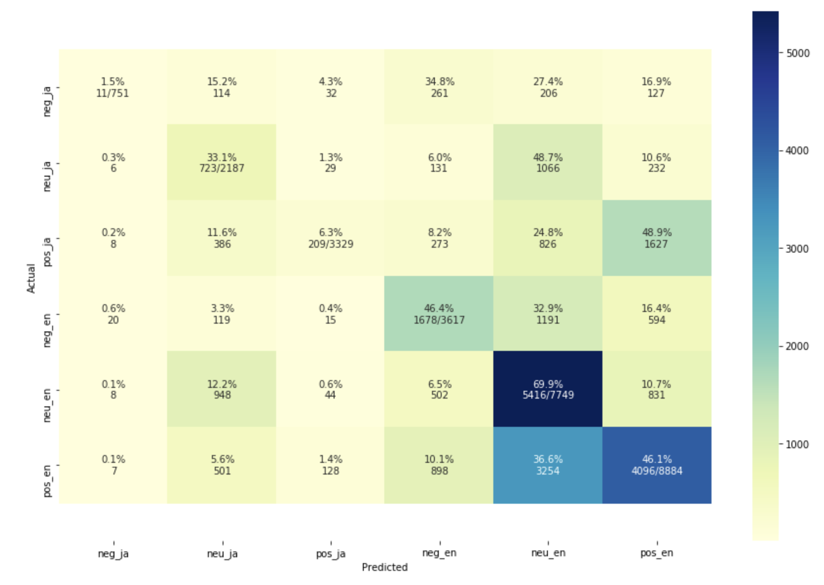
• I collected 26000 tweets for the 2020 CNY about Disney using the above model.

• However, understandably since it’s another seasonal holiday
  • The random forest model scored 46 percent accuracy
  • The multinomial bayes classifier scored only 33 percent accuracy

• Halloween data is another holiday compared to Chinese New Year. Therefore, words used during the tweets would be different. Furthermore, 3 main events were happening around this time.

  • Kobe’s death
  • Coronavirus
  • Super Bowl

Disney NLP full write up

Disney NLP Github link